Hadley Wickham的ggplot2 是一个出色且灵活的包,用于在 R 中进行优雅的数据可视化。但是,默认生成的图需要一些格式才能发送它们以供发布。 此外,要自定义 ggplot,语法是负责的,这提高了没有高级 R 编程技能的研究人员的难度。
ggpubr包 提供了一些易于使用的功能,可以使用更简单的语法代码绘制出可供发表出版的图表。
安装
install.packages("ggpubr")
## 折线图
library(ggpubr)

df <- data.frame(supp=rep(c("VC", "OJ"), each=3),
   dose=rep(c("D0.5", "D1", "D2"),2),
   len=c(6.8, 15, 33, 4.2, 10, 29.5))
#print(df)
#>   supp dose  len
#> 1   VC D0.5  6.8
#> 2   VC   D1 15.0
#> 3   VC   D2 33.0
#> 4   OJ D0.5  4.2
#> 5   OJ   D1 10.0
#> 6   OJ   D2 29.5

# Plot "len" by "dose" and
# Change line types and point shapes by a second groups: "supp"
ggline(df, x="dose", y="len",
  linetype = "supp", shape = "supp")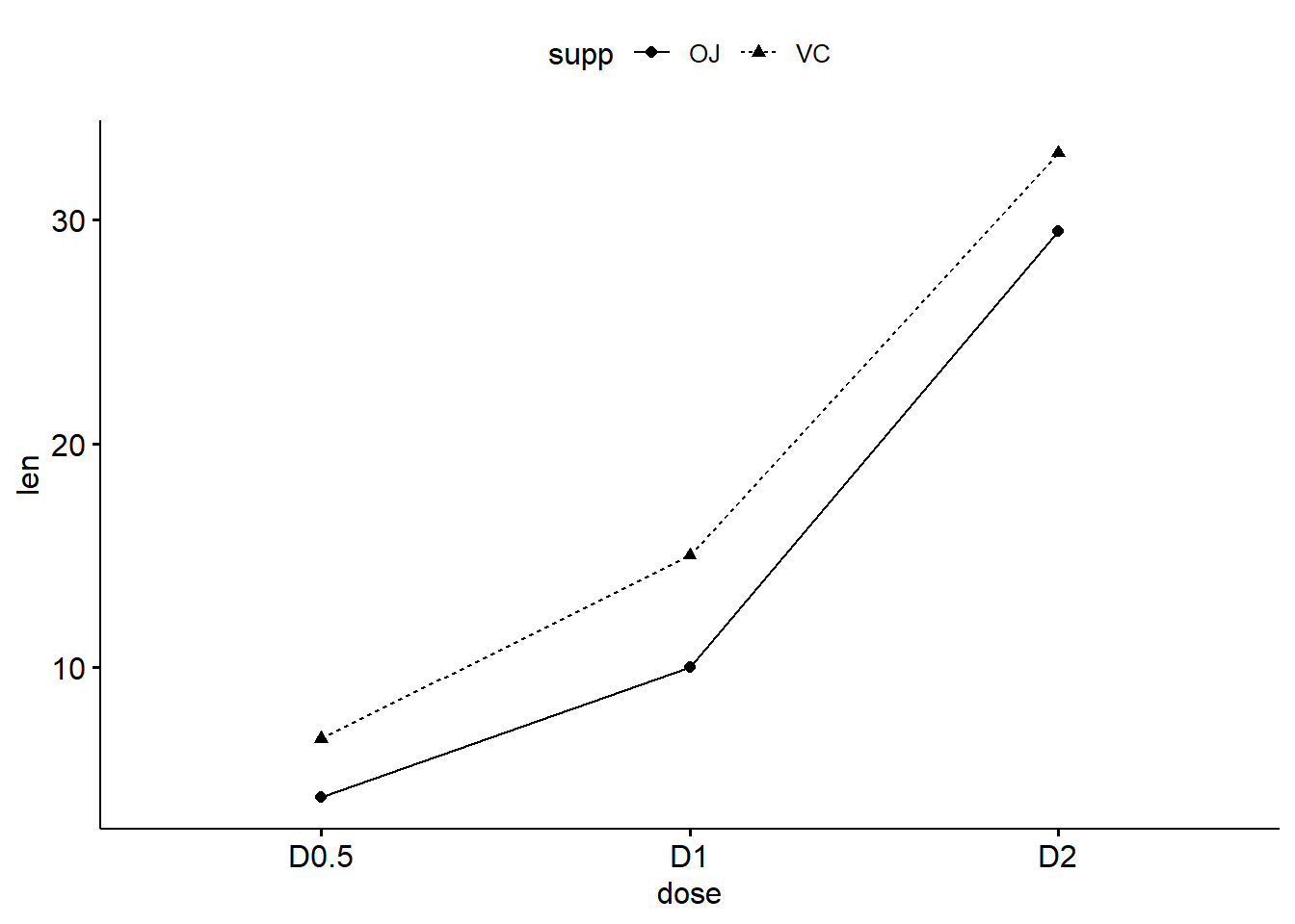
# Change colors
# +++++++++++++++++++++

# Change color by group: "supp"
# Use custom color palette
ggline(df, x="dose", y="len",
   linetype = "supp", shape = "supp",
   color = "supp", palette = c("#00AFBB", "#E7B800"))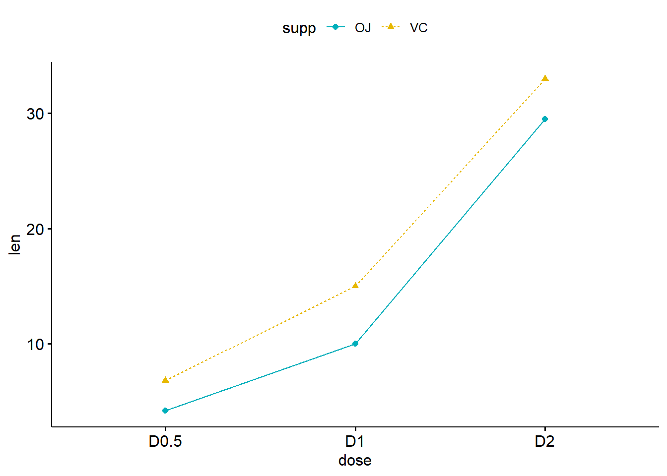
散点图
# Load data
data("mtcars")
df <- mtcars
df$cyl <- as.factor(df$cyl)
#head(df[, c("wt", "mpg", "cyl")], 3)
#>                  wt  mpg cyl
#> Mazda RX4     2.620 21.0   6
#> Mazda RX4 Wag 2.875 21.0   6
#> Datsun 710    2.320 22.8   4

# Textual annotation
# +++++++++++++++++
df$name <- rownames(df)
ggscatter(df, x = "wt", y = "mpg",
   color = "cyl", palette = c("#00AFBB", "#E7B800", "#FC4E07"),
   label = "name", repel = TRUE)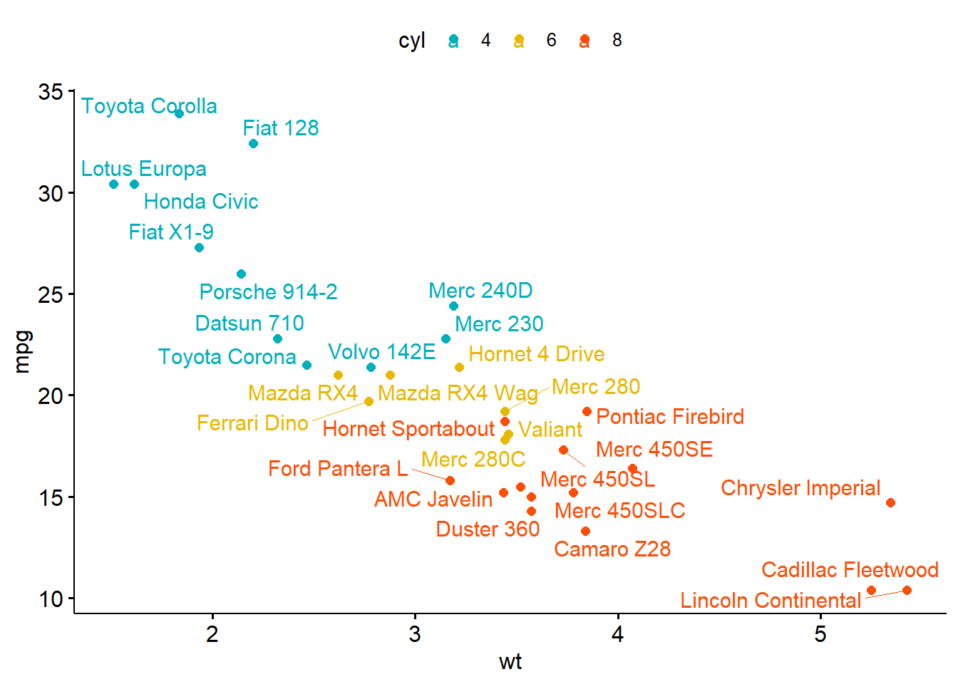
饼形图
df <- data.frame(
 group = c("Male", "Female", "Child"),
  value = c(25, 25, 50))

#head(df)
#>    group value
#> 1   Male    25
#> 2 Female    25
#> 3  Child    50


# Basic pie charts
# ++++++++++++++++++++++++++++++++

ggpie(df, "value", label = "group")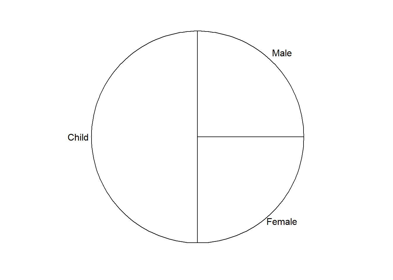
ggpie(df, "value", label = "group", fill="group")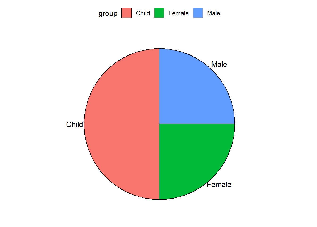
ggpie(df, "value", label = "group", fill="group", color='white')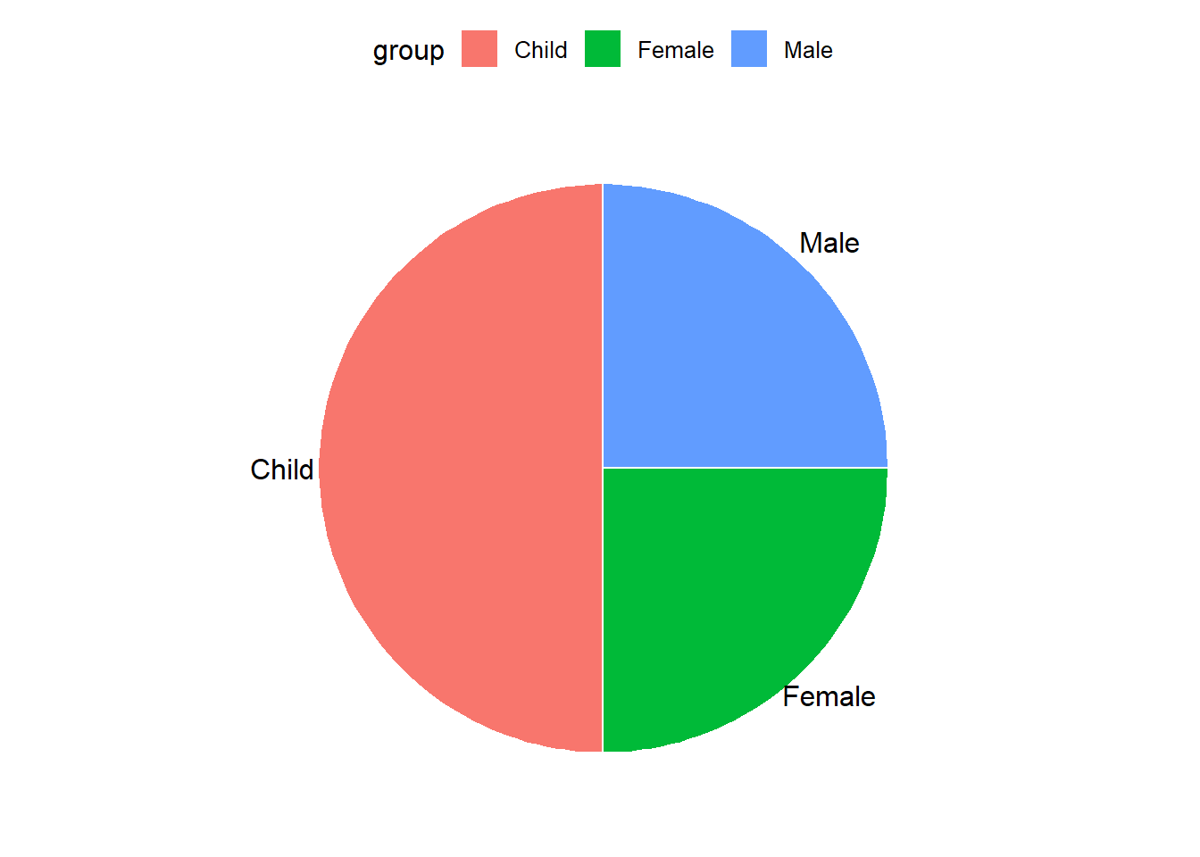
ggpie(df, "value", label = "group", fill="group",
      palette = c("#00AFBB", "#E7B800", "#FC4E07"),
      color='white')
labs <- paste0(df$group, " (", df$value, "%)")
#> "Male (25%)"   "Female (25%)" "Child (50%)"

ggpie(df, "value", label = labs, fill="group",
      palette = c("#00AFBB", "#E7B800", "#FC4E07"),
      color='white')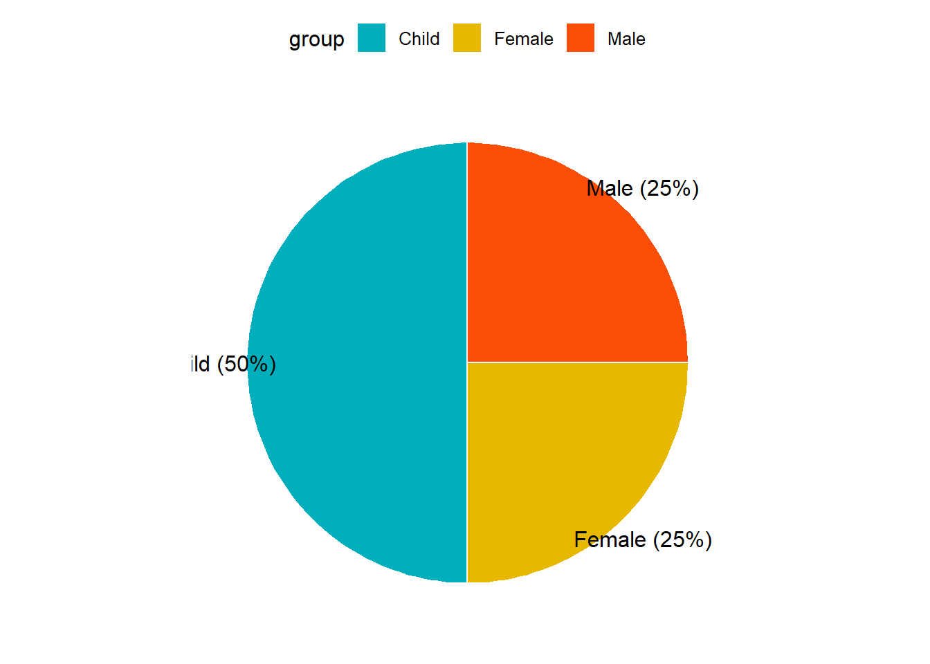
labs <- paste0(df$group, " (", df$value, "%)")
#> "Male (25%)"   "Female (25%)" "Child (50%)"

ggpie(df, "value", label = labs, fill="group",
      lab.pos = "in", lab.font = "white",
      palette = c("#00AFBB", "#E7B800", "#FC4E07"),
      color='white')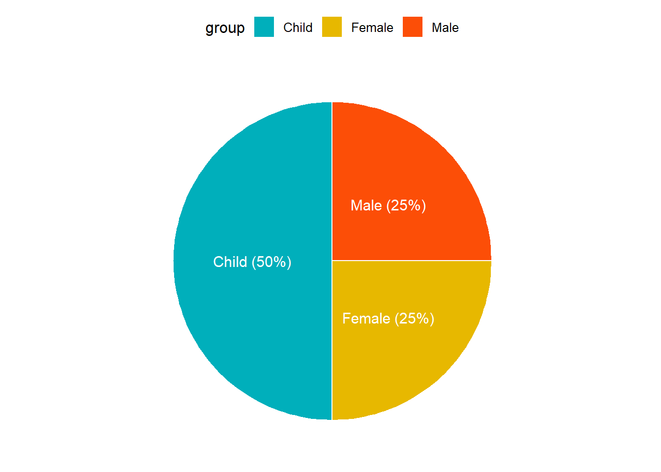
甜甜圈图
#> head(df)
#>    group value
#> 1   Male    25
#> 2 Female    25
#> 3  Child    50
#>
# Change the position and font color of labels
ggdonutchart(df, "value", label = labs,
   lab.pos = "in", lab.font = "white",
   fill = "group", color = "white",
   palette = c("#00AFBB", "#E7B800", "#FC4E07"))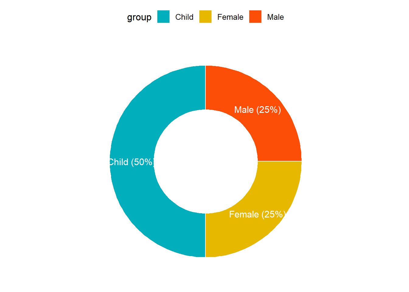
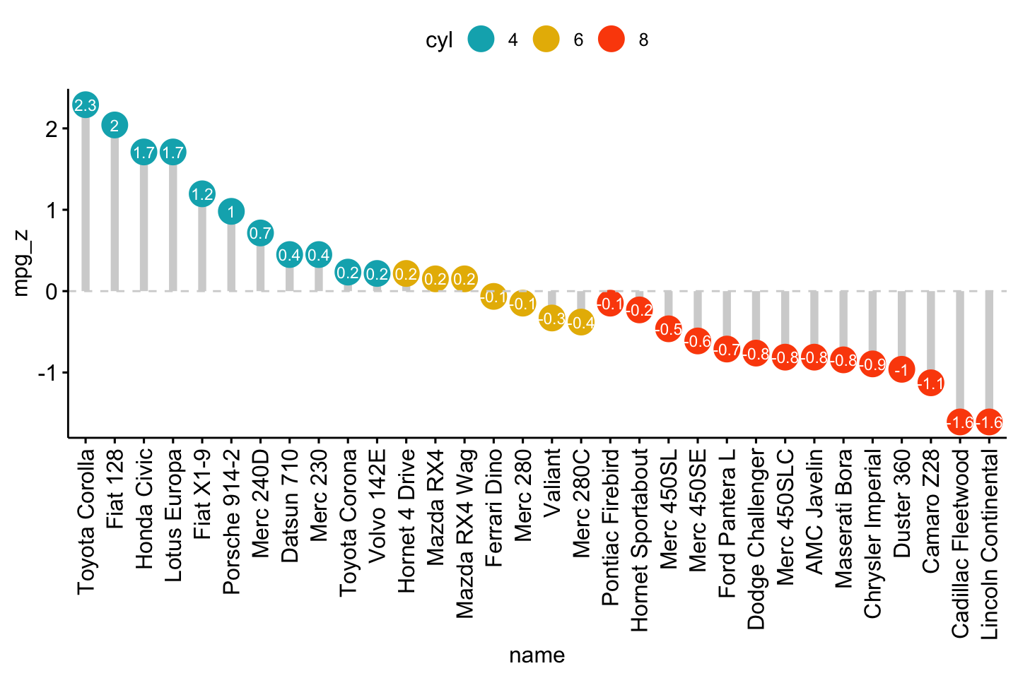
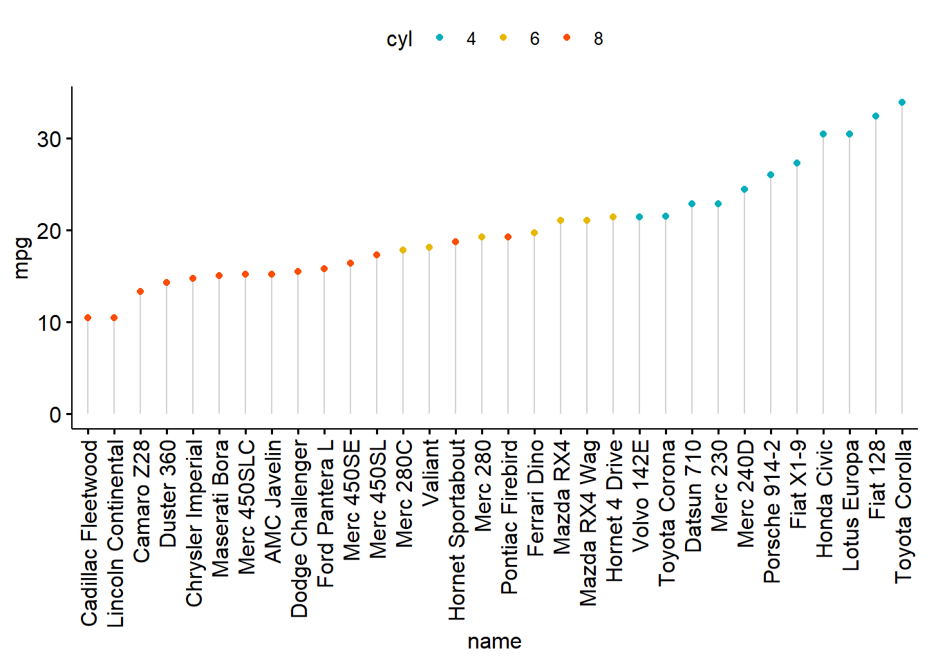
点图
# Load data
data("mtcars")
dfm <- mtcars
# Convert the cyl variable to a factor
dfm$cyl <- as.factor(dfm$cyl)
# Add the name colums
dfm$name <- rownames(dfm)
# Inspect the data
#head(dfm[, c("name", "wt", "mpg", "cyl")])
#>                                name    wt  mpg cyl
#> Mazda RX4                 Mazda RX4 2.620 21.0   6
#> Mazda RX4 Wag         Mazda RX4 Wag 2.875 21.0   6
#> Datsun 710               Datsun 710 2.320 22.8   4
#> Hornet 4 Drive       Hornet 4 Drive 3.215 21.4   6
#> Hornet Sportabout Hornet Sportabout 3.440 18.7   8
#> Valiant                     Valiant 3.460 18.1   6

ggdotchart(dfm, x = "name", y = "mpg",
           color = "cyl",                                # Color by groups
           palette = c("#00AFBB", "#E7B800", "#FC4E07"), # Custom color palette
           sorting = "ascending",                        # Sort value in descending order
           add = "segments",                             # Add segments from y = 0 to dots
           ggtheme = theme_pubr()                        # ggplot2 theme
           )
密度图
set.seed(1234)
wdata = data.frame(
   sex = factor(rep(c("F", "M"), each=200)),
   weight = c(rnorm(200, 55), rnorm(200, 58)))
#head(wdata, 4)
#>   sex   weight
#> 1   F 53.79293
#> 2   F 55.27743
#> 3   F 56.08444
#> 4   F 52.65430

# Density plot with mean lines and marginal rug
# :::::::::::::::::::::::::::::::::::::::::::::::::::
# Change outline and fill colors by groups ("sex")
# Use custom palette
ggdensity(wdata, x = "weight", color='sex')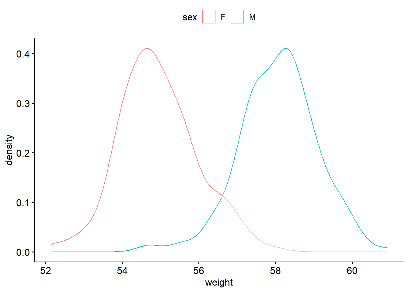
ggdensity(wdata, x = "weight", color='sex', add='mean')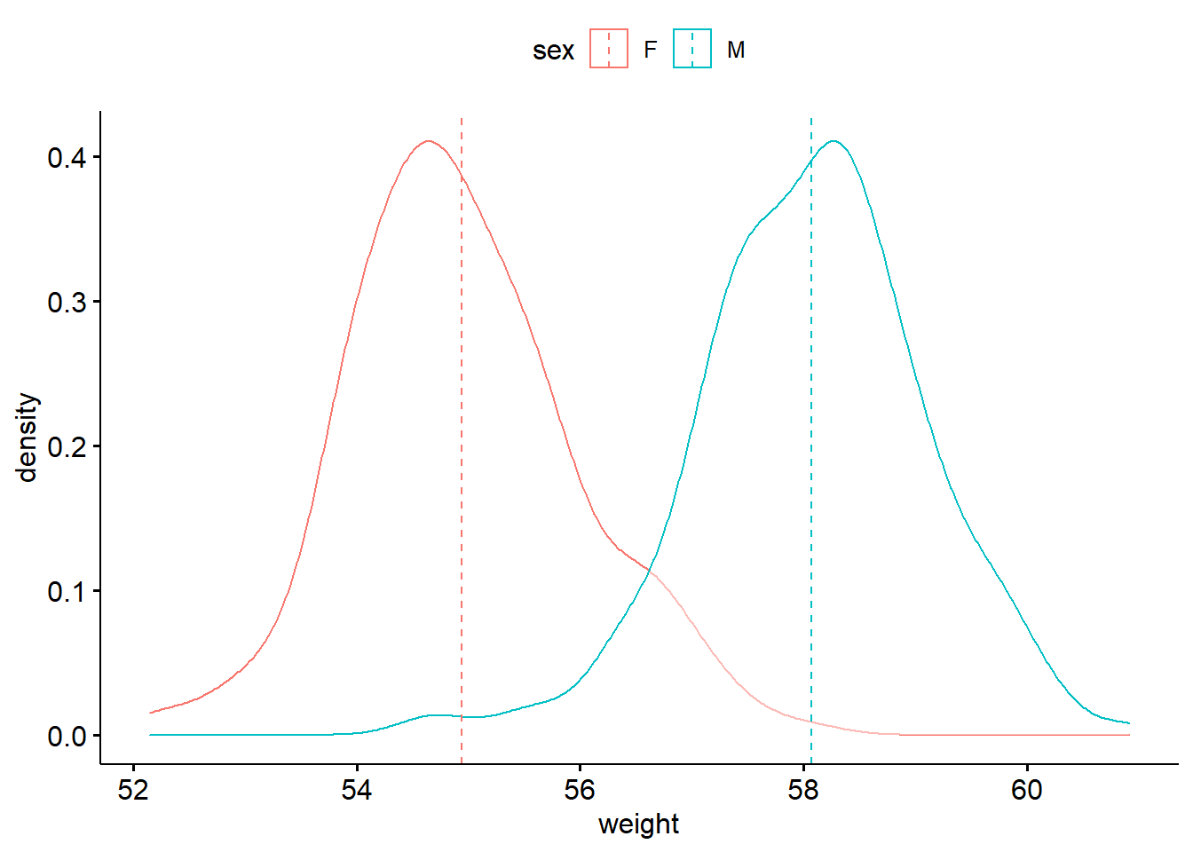
ggdensity(wdata, x = "weight", color='sex', add='mean', rug=TRUE)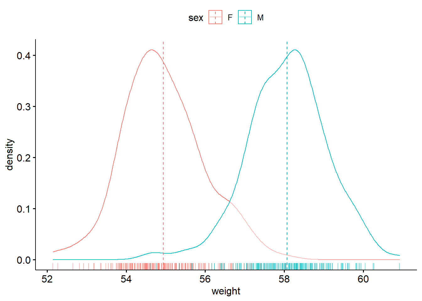
ggdensity(wdata, x = "weight", color='sex', add='mean', rug=TRUE, fill='sex')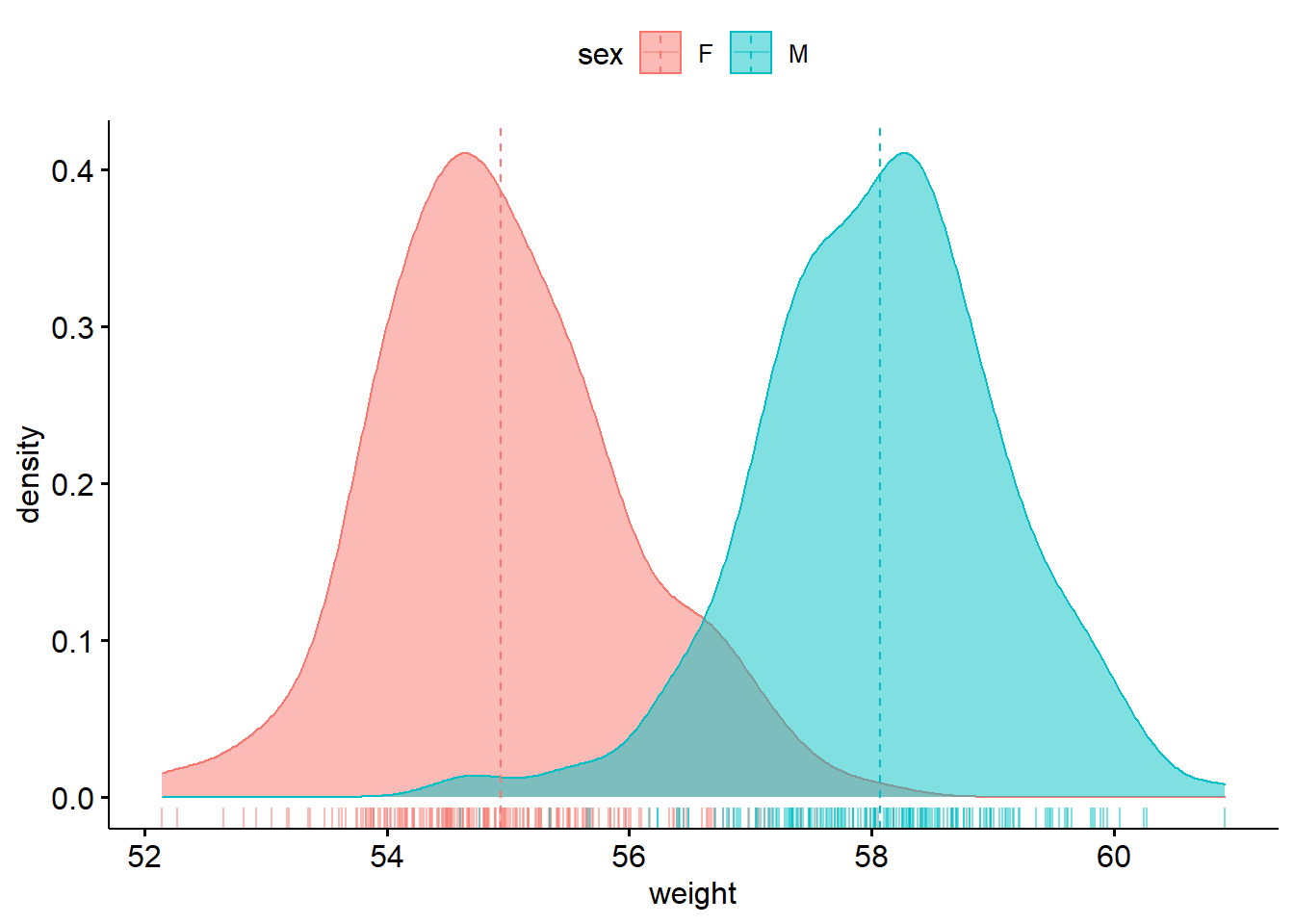
ggdensity(wdata, x = "weight", color='sex', add='mean', rug=TRUE, fill='sex',
          palette = c("#00AFBB", "#E7B800"))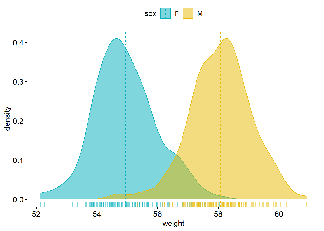
直方图
# Histogram plot with mean lines and marginal rug
# :::::::::::::::::::::::::::::::::::::::::::::::::::
# Change outline and fill colors by groups ("sex")
# Use custom color palette
gghistogram(wdata, x = "weight",
   add = "mean", rug = TRUE,
   color = "sex", fill = "sex",
   palette = c("#00AFBB", "#E7B800"))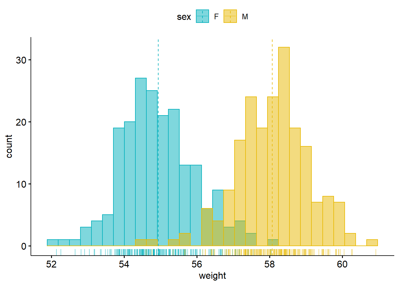
箱图
# Load data
data("ToothGrowth")
df <- ToothGrowth
#head(df, 4)
#>    len supp dose
#> 1  4.2   VC  0.5
#> 2 11.5   VC  0.5
#> 3  7.3   VC  0.5
#> 4  5.8   VC  0.5

# Box plots with jittered points
# :::::::::::::::::::::::::::::::::::::::::::::::::::
# Change outline colors by groups: dose
# Use custom color palette
# Add jitter points and change the shape by groups
 p <- ggboxplot(df, x = "dose", y = "len", add = "jitter",
                color = "dose", shape = "dose",
                palette =c("#00AFBB", "#E7B800", "#FC4E07"))
 p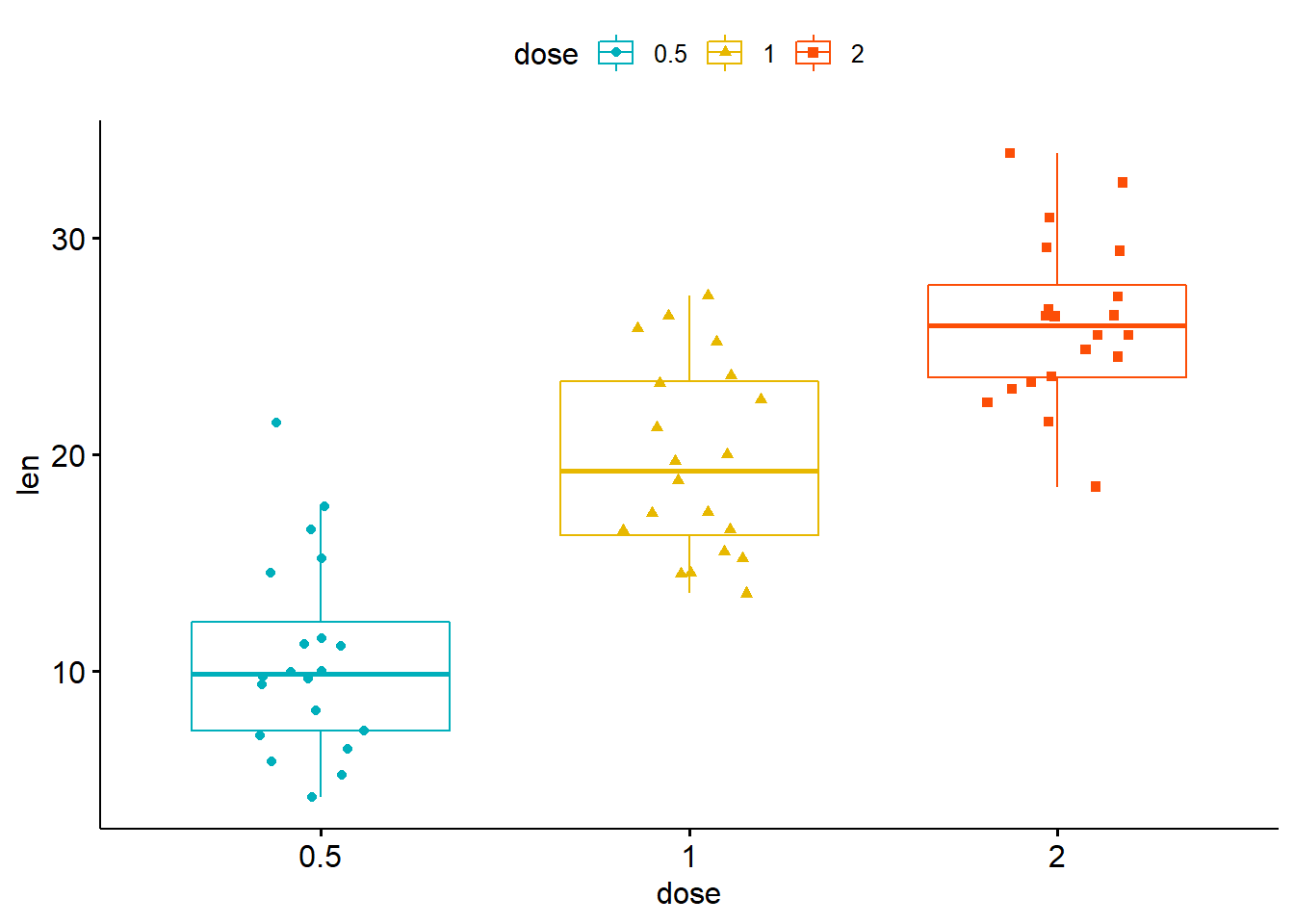
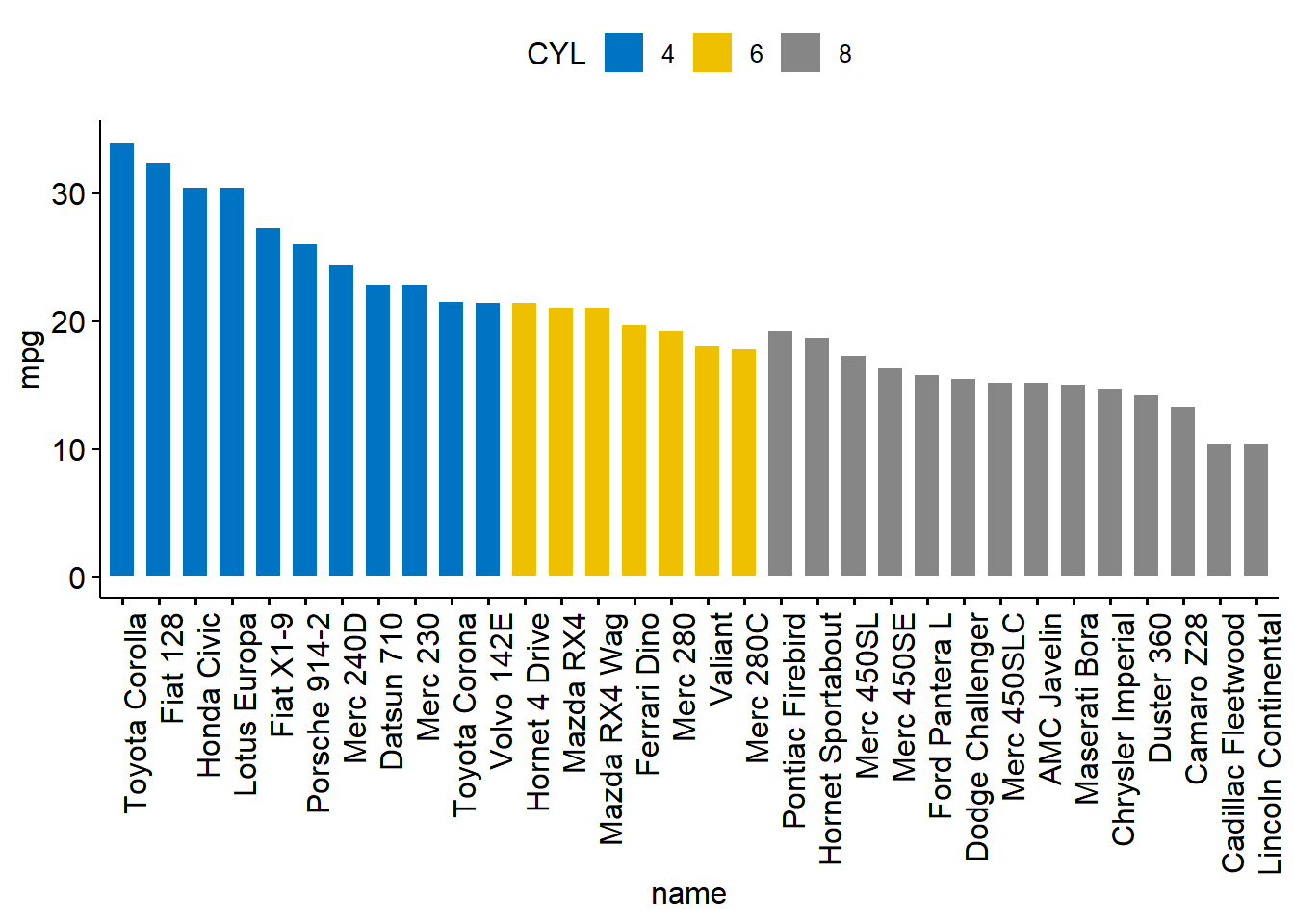
条形图
# Load data
data("mtcars")
dfm <- mtcars
# Convert the cyl variable to a factor
dfm$cyl <- as.factor(dfm$cyl)
# Add the name colums
dfm$name <- rownames(dfm)
# Inspect the data
#head(dfm[, c("name", "wt", "mpg", "cyl")])
#>                                name    wt  mpg cyl
#> Mazda RX4                 Mazda RX4 2.620 21.0   6
#> Mazda RX4 Wag         Mazda RX4 Wag 2.875 21.0   6
#> Datsun 710               Datsun 710 2.320 22.8   4
#> Hornet 4 Drive       Hornet 4 Drive 3.215 21.4   6
#> Hornet Sportabout Hornet Sportabout 3.440 18.7   8
#> Valiant                     Valiant 3.460 18.1   6

ggbarplot(dfm, x = "name", y = "mpg",
          fill = "cyl",               # change fill color by cyl
          color = "white",            # Set bar border colors to white
          palette = "jco",            # jco journal color palett. see ?ggpar
          sort.val = "desc",          # Sort the value in dscending order
          sort.by.groups = TRUE,      # Sort inside each group
          x.text.angle = 90           # Rotate vertically x axis texts
          )
ggbarplot(dfm, x = "name", y = "mpg",
          fill = "cyl",               # change fill color by cyl
          color = "white",            # Set bar border colors to white
          palette = "jco",            # jco journal color palett. see ?ggpar
          sort.val = "desc",          # Sort the value in dscending order
          sort.by.groups = TRUE,      # Don't sort inside each group
          x.text.angle = 90,          # Rotate vertically x axis texts
          legend.title = "CYL"        # Set legend title
          )
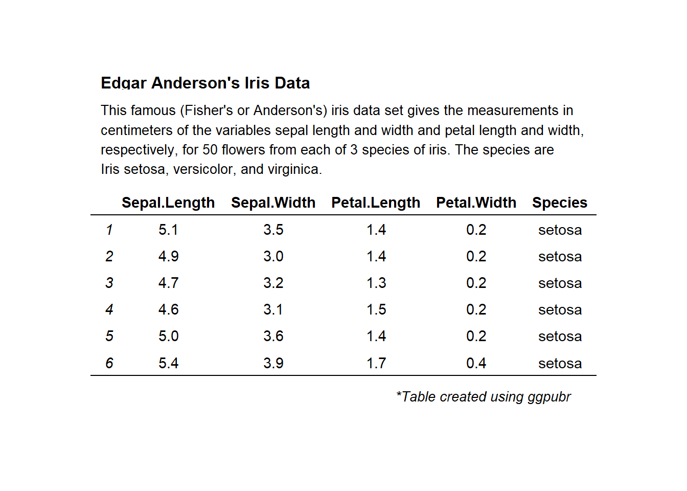
表格
#Medium blue (mBlue) theme
ggtexttable(head(iris), rows = NULL, theme = ttheme("mBlue"))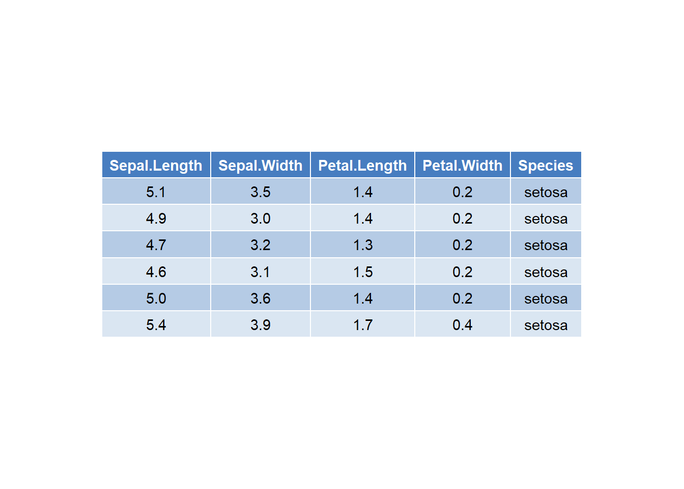
main.title <- "Edgar Anderson's Iris Data"
subtitle <- paste0(
"This famous (Fisher's or Anderson's) iris data set gives the measurements",
" in centimeters of the variables sepal length and width and petal length and width,",
 " respectively, for 50 flowers from each of 3 species of iris.",
 " The species are Iris setosa, versicolor, and virginica."
) %>%
 strwrap(width = 80) %>%
 paste(collapse = "\n")

tab <- ggtexttable(head(iris), theme = ttheme("light"))
tab %>%
 tab_add_title(text = subtitle, face = "plain", size = 10) %>%
 tab_add_title(text = main.title, face = "bold", padding = unit(0.1, "line")) %>%
 tab_add_footnote(text = "*Table created using ggpubr", size = 10, face = "italic")